How to model material plasticity in Abaqus
Almost all the materials show elastic behavior in a period and then plastic behavior and permanent deformations take place. This is what we see in the tensile test results. So, as a finite element user it is important to know how to model material plasticity in Abaqus. The purpose of this post is to getting familiar with materials plastic properties and its modeling approach in Abaqus.
Tutoring finite element analysis is the main goal of this websites post. Thus, in most of the examples simple geometries are implemented and we will not spend a lot of time for preparing parts’ geometries.
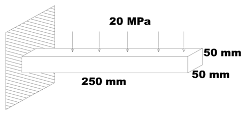
A cantilever beam with distributes load on its top surface is the example bieng chosen for this tutoring post. The beam dimensions, loading and boundary conditions are depicted in the figure.
Material properties are stated in ‘Property mdule’ section.
Part/Sketch
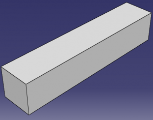
In the ‘Part’ module create a ‘250×50’ sketch and extrode it for 25 mm.
Property
The material plastic properties are the most important section of this post. Like other examples material density, Young modulus and Poisson ratio should be entered in the ‘create material’ window.
Density = 7800 Kg/M3
Young’s Module = 200 GPa
Poisson’s Ratio = 0.3
These properties represent the material behavior in the elastic region. But, after the yield strain the material behavior is not linear any more. Thus, entering other complimentary material data is necessary. One can obtain material plastic behavior from tension test results. In this example stress and strain data are extracted from one type of steel tesion test.
It is of greate importance to notice that tension test data are ‘nominal’ or ‘engineering’ results. To use them in Abaqus one first must convert them to ‘true’ values using these equations:
ε = ln (1+ε0)
σ = σ0 (1+ε0)
where ε0 and σ0 are nominal strain and stress, ε and σ are true strain and stress respectively.
According to this point, obtained stress and strain data from the test are converted to true values as seen in the table and plot.
| stress(MPa( | strain | plastic strain |
| 0 | 0 | |
| 538 | 0.00269 | 0 |
| 559 | 0.006632 | 0.003942 |
| 631 | 0.029961 | 0.027271 |
| 679 | 0.041425 | 0.038735 |
| 753 | 0.060243 | 0.057553 |
| 835 | 0.086008 | 0.083318 |
| 878 | 0.11112 | 0.10843 |
| 918 | 0.13216 | 0.12947 |
| 960 | 0.15277 | 0.15008 |
| 1005 | 0.17628 | 0.17359 |
| 1022 | 0.19274 | 0.19005 |
| 1035 | 0.20572 | 0.20303 |
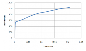
In the table first column is the true stress, second column is the true strain and the third column is plastic strain which is determined by taking yield strain from true strain.
εplastic = ε-εyield
First and third columns should be entered in Abaqus material properties as shown in the figure.
Mechanical / Plasticity / Plastic

Enter tha table values in the ‘create material’ window.
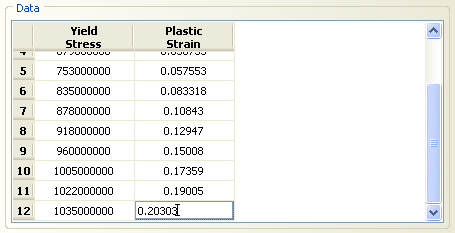
Pay attention to the units; Stress should be entered as Pascal, so e+6 at the end of each value is necessary.
Step
You can do the other levels of the model creation like what you have learnt from the other examples. Notice that because we want to study the non-linear behavior of material, NLGeom option in the ‘create step’ window should be activated.
As we want to plot some diagrams for the boundary conditions, in ‘step’ module a ‘History output’ should be defined. Stresses and strains will be stored.
To define ‘History output’, first a ‘set’ must be defined for the desired region. From the ‘main menu’ select set creation:
Tools / Set / Create
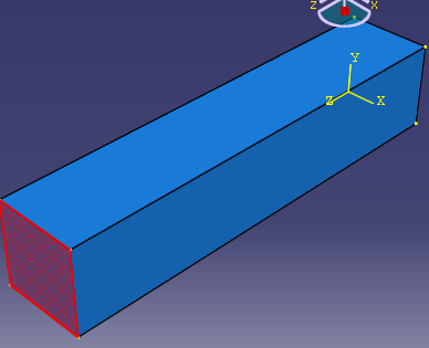
and then select the beam base, name it ‘Base’ and click on OK.
After defining the set, click on the ‘History output manager’ and delete the existing ‘H-Output-1’ since we don’t need it. Now create a new History output and do the following configurations:
Domain: Set : Base
Frequency: Evenly Spaced Time Intervals : 100
Output Variables: EP, SP,
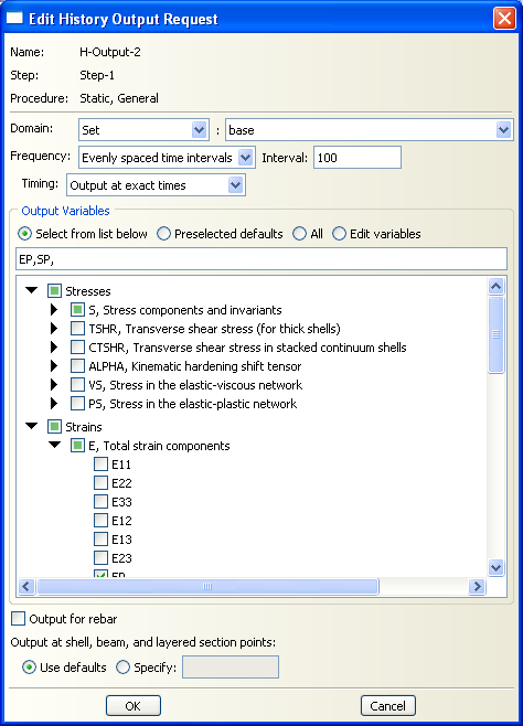
Indeed, we ask Abaqus to only record ‘Principal Stress & Strain’. We asked Abaqus to do not record any other History values because then in the results section, Visualization module, it will be a little difficult to find the desired results when there are some other undesired recorded results .
Load
Apply the pressure load on the beam top surface and fix one of the beam ends.
Load: Mechanical / Pressure : 20 E+6
Mesh
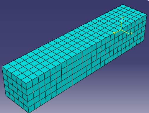
In the Mesh module seed the model by 0.01 units and use structured Hex elements to mesh it as depicted.
Job
In Job module you need to create a job, neme it ‘Plasticity’ and then submit it. You may click on ‘Monitor’ button to see the analysis process.
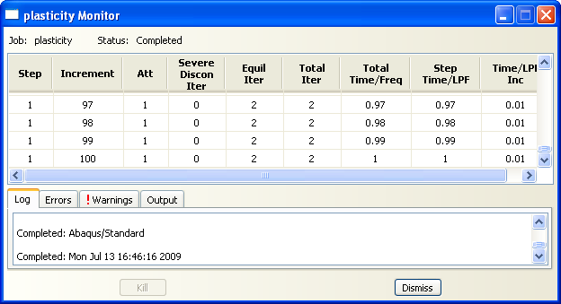
It is important to understand the meaning of the ‘time’ shown in monitor window or in the plots. In dynamic simulation time is the time and its unit is something like seconds or milliseconds or so; but, in static simulation what shown as time is actually the percentage of the analysis. For example if the total applying load is 100 N, then time=0.25 means that at this moment 25% of the load has been applied. Indeed, in static simulations load is applied gradually in very small steps, so there would be no inertial force. That’s why in the load window in front of the ‘Amplitude’, the default choice is ‘Ramp’ which means the total load will be applied gradually and it is exactly the meaning of the static phenomenon.
Visualization
The results of the simulation are shown in the ‘Visualization’ module. If you want to see the results from different angles or studying different outputs at the same time, you can create new ‘Viewport’ from the main menu:
Viewport / Create
By doing so a new ‘viewport’ will be created. To see that viewport side-by-side the current viewport you have some ‘Tile’ options under the ‘Viewport’ command in the main menu bar. For example to tile them vertically click on ‘Tile Vertically’:
Viewport / Tile Vertically
Now, show ‘Mises’ output in one and Principal Strain, ‘PE’, in the other one.

As seen in the figure, although stress is distributed in the entire beam, plastic strain or permanent deformation only happened at the fixing area. In the left figure areas which are shown as blue are still in the elastic region.
In this example we’ll get familiar with other Abaqus abilities to plot curves. One of these very useful and applicable abilities is to plot to different outputs against each other. For example in this example we will plot the stress-strain curve. As you have experienced, by default Abaqus plot output curves versus time.
To do so first we need to know the number of one of the elements which experiencing plastic deformation. From the main menu run ‘Query’ command:
Tools / Query
You also have access to this command through the ‘i’ button in the toolbar. In the Query window select ‘Element’ and select the element shown in the figure from the viewport.
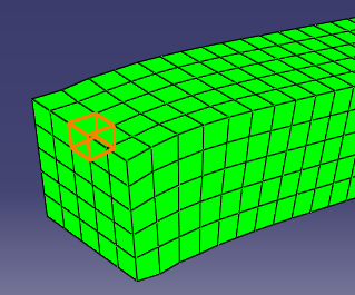
The element number will be shown at the bottom of the viewport and may vary in your computer. Here the element number is 503.
![]()
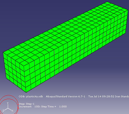
Now, first we will plot the principal stress along the beam axis. Here the beam access is the ‘Z’ axis. Depends on the part creation or the part assembly the beam axis in your system may vary. To find it out pay attention to the coordinate system shown in the viewport. It is highlighted in the figure.
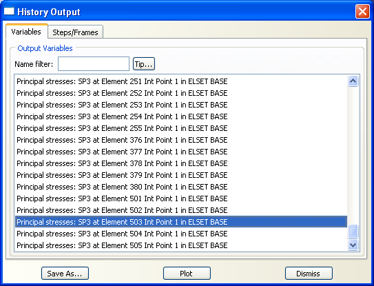
I need to plot principal stress along the ‘Z’, 3rd, direction. Thus, I will select ‘SP3 at element 503’ from the history output window and click ‘Plot’ and ‘Save as’. Stress vs. Time curve will be plotted.
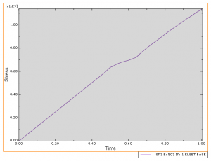
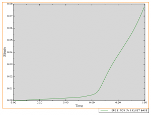
We need to repeat this part and plot the principal strain for element 503 as well. So, select ‘EP3 for element 503’ from the history output window and click ‘Plot’ and ‘Save as’.
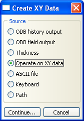
Click on the ‘Creat XY Data’ icon from the toolbar again and select ‘Operate on XY Data’.
If you are done the previous steps correctly, plotting and saving curves, the ‘operate on XY Data’ window should be alike this:
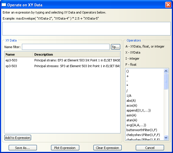
This window contains three major parts. The top window is for entering equations by the user. The ‘XY Data’ section contains the curves stored and saved by the user. In this example we have saved 2 curves, EP3 and SP3 for element 503, which can be seen in the window. The ‘Operators’ section involves a variety of mathematical and statistical operations such as +, – , *, sin, cos and so on. User can exploit these operators and apply them on the available analysis results to define his own desired curve.
To plot stress-strain curve we need to combine stress-time and strain-time curves together. The ‘Combine(X,X)’ operator can do this. So, select ‘Combine(X,X)’ from the operators list. The first variable would be the x-axis and the second would be the y-axis. First, select EP3 from the XY Data and click ‘Add to Expression’ button. Next, do the same for SP3.
The equation shown in the top box is something like this depending on the element number:
Combine ( “Ep3-503”, “Sp3-503”)
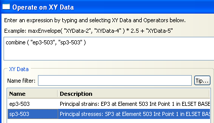
Click on ‘Plot Expression’ so that the stress-strain curve be plotted.
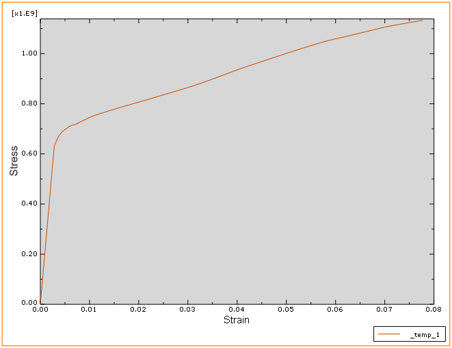
As we expected this curve must be the stress-strain curve which we had introduced in the Property module.

